Disclaimer
The information and the links provided are for general information only and should not be taken as constituting professional advice.
I am not liable for any loss caused, whether due to negligence or otherwise arising from the use of, or reliance on, the information provided directly or indirectly on this post.
Introduction
With Python, this post demonstrates how to :
- Import price data
- Simulate a simple moving average strategy
- Compare performance with a hodling strategy
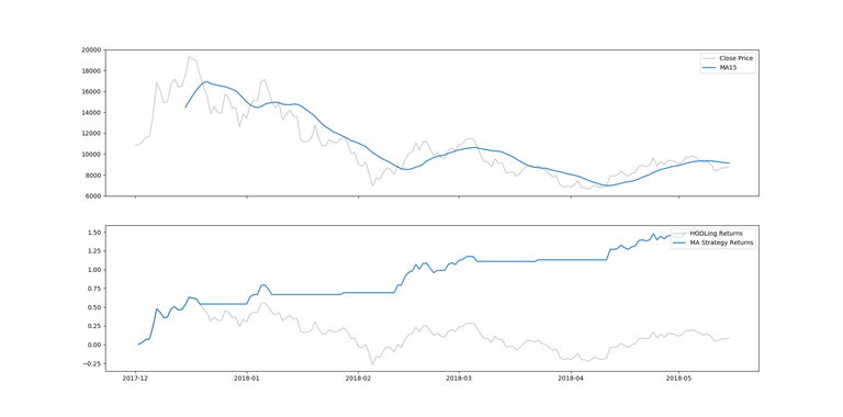
You will be able to reproduce the following figure:

The first graph displays in gray the BTC/USD closing price between December 1st, 2017 and May 15th, 2018. The blue line plots the 15 days moving average. Any point on the blue line is the average closing price over the 15 previous days.
The second graph compares a simple moving average strategy (blue) to a hodling strategy (gray). A simple moving average strategy consists in buying and hodling when the closing price is above a moving average. As soon as the moving average is above the closing price, it’s time to sell and wait for the next buying signal.
The 15-days moving average strategy would have generated 130% return on investment from December 1st, 2017 until May 15th, 2018. In contrast, hodling provided 8% return of investment despite a correction in January 2018.
Just give me the code !
import pandas as pd
import numpy as np
import datetime as dt
import matplotlib.pyplot as plt
import talib as t


# Get historical data
df = pd.read_csv('coindesk-bpi-USD-close_data-2017-12-01_2018-05-15.csv', skipfooter=2)

# Calculate moving averages
df['MA15'] = t.MA(np.array(df['Close Price']), timeperiod=15)

# Find trading signals
df['Signal'] = 1
df.loc[(df['MA15'] > df['Close Price']), 'Signal'] = 0

# Calculate returns
df['HODLing Returns'] = (df['Close Price'] - df['Close Price'].shift(1)) / df['Close Price'].shift(1)
df['MA Strategy Returns'] = df['Signal'] * df['HODLing Returns']

# Plots
dates = df['Date'][:len(df['Close Price'])]
dates = [dt.datetime.strptime(d, '%Y-%m-%d %H:%M:%S').date() for d in dates]
fig, axes = plt.subplots(2, 1, sharex=True)
axes = axes.flatten()

axes[0].plot(dates, df['Close Price'], lw=1, alpha=0.6, color='grey')
axes[0].plot(dates, df['MA15'], lw=2, alpha=0.8)
axes[0].legend(loc='upper right')

axes[1].plot(dates, df['HODLing Returns'].cumsum(), lw=1, alpha=0.6, color='grey')
axes[1].plot(dates, df['MA Strategy Returns'].cumsum(), lw=2, alpha=0.8)
axes[1].legend(loc='upper right')

plt.show()
Importing data
I have downloaded BTC/USD closing price from December 1st, 2017 to May 15th, 2018 on coindesk. Just choose a time period to analyze, click on 'Export' and click on 'Download CSV Chart Data'.
Make sure that the csv file and the python script are in the same folder. Then, importing data in Python takes two lines:
import pandas as pd
df = pd.read_csv('coindesk-bpi-USD-close_data-2017-12-01_2018-05-15.csv', skipfooter=2)
The argument skipfooter=2 skips the two last rows. Why? Coindesk adds 2 lines at the end of their file that are useless for the analysis.
To have a look at the first observations, run print(df.head()).
Moving average
I love using the library TA-Lib to calculate financial indicators. Not only does it include moving averages but also MACD, RSI, Bollinger Bands, and more.
The following calculates a 15-periods Moving Average of the Closing Price:
import talib as t
import numpy as np
df['MA15'] = t.MA(np.array(df['Close Price']), timeperiod=15)
Buying signals
df['Signal'] = 1
df.loc[(df['MA15'] > df['Close Price']), 'Signal'] = 0
The first line initializes the signal to 1. It says, 'you should hodl Bitcoin'. Then, the second line sets the signal to 0 when the MA is greater than the closing price.
In other words, if the signal changes from 0 to 1, it's time to buy; if the signal changes from 1 to 0, it's time to sell.
Calculating returns
df['HODLing Returns'] = np.log(df['Close Price'] / df['Close Price'].shift(1))
df['MA Strategy Returns']  = df['Signal'] * df['HODLing Returns']
The first line calculates daily returns on investment when hodling BTC/USD.
The second line calculates daily returns from the MA strategy defined earlier.
Plotting
import datetime as dt
import matplotlib.pyplot as plt

dates = df['Date'][:len(df['Close Price'])]
dates = [dt.datetime.strptime(d, '%Y-%m-%d %H:%M:%S').date() for d in dates]

fig, axes = plt.subplots(2, 1, sharex=True)
axes = axes.flatten()

axes[0].plot(dates, df['Close Price'], lw=1, alpha=0.6, color='grey')
axes[0].plot(dates, df['MA15'], lw=2, alpha=0.8)
axes[0].legend(loc='upper right')
axes[1].plot(dates, df['HODLing Returns'].cumsum(), lw=1, alpha=0.6, color='grey')
axes[1].plot(dates, df['MA Strategy Returns'].cumsum(), lw=2, alpha=0.8)
axes[1].legend(loc='upper right')
plt.show()
The first plot, defined by axes[0], represents the price action and the moving average.
The second plot gives the cumulative returns of both the Moving Average strategy (blue), and the hodling strategy (grey). It reproduces the figure at the beginning of the post.

Concluding Remarks
It is too good to be true, isn’t? Probably. Backtests tell what would have happened if you have had followed this strategy. There is no guarantee that the strategy will outperform the market in the future.
Finding the right Moving Average is more an art that a science. If you apply the same methodology to any other currency and time frame, it will require trials and errors to spot a Moving Average that fits a profitable strategy.
Moreover, Moving Averages are rather rudimentary tool. Additional indicators (like the MACD), critical thinking and reactivity are crucial when it comes to implementing trading strategies.
Future posts:
- Automating a moving average strategy on Binance
- Triangular arbitrage strategy
- Twitter sentiment analysis for trading on cryptos (certainly on Verge)
Want to see a specific indicator? A specific currency? Any other requirement for a future post? Feel free to ask in the comments.
Congratulations @grayble! You have completed some achievement on Steemit and have been rewarded with new badge(s) :
Click on any badge to view your own Board of Honor on SteemitBoard.
For more information about SteemitBoard, click here
If you no longer want to receive notifications, reply to this comment with the word
STOPCongratulations @grayble! You have completed some achievement on Steemit and have been rewarded with new badge(s) :
Click on any badge to view your Board of Honor.
For more information about SteemitBoard, click here
If you no longer want to receive notifications, reply to this comment with the word
STOPDo not miss the last announcement from @steemitboard!
Congratulations @grayble! You received a personal award!
Click here to view your Board
Do not miss the last post from @steemitboard:
Vote for @Steemitboard as a witness and get one more award and increased upvotes!
Congratulations @grayble! You received a personal award!
You can view your badges on your Steem Board and compare to others on the Steem Ranking
Do not miss the last post from @steemitboard:
Vote for @Steemitboard as a witness to get one more award and increased upvotes!