
The image above was made with stable diffusion using the prompt 'a futuristic robot trading crypto.'
A few years back, I spent an immense amount of time trying to make a bot that traded better than I could trade manually. I spent countless hours attempting to predict prices with LSTM and other kinds of neural networks, but my results were always mixed at best. This year, I picked the project up again. After throwing all of my old assumptions out the window and starting from scratch, I finally devised an algo with real potential.
Wrangling Data
To start, I needed data. Historical trade data has always been hard to come by unless you want to pay Coinmarketcap's insane api prices, but I managed to find a year's worth of OHLCV data on CHEX and EOS here. A tiny script turned scraped data into a couple of clean csv files. Then I used mpl finance to plot the CHEX and EOS candlesticks like this.
import pandas as pd
import mplfinance as mpf
import matplotlib.pyplot as plt
from matplotlib.lines import Line2D  # For custom legend elements

# File paths
chex_filepath = "C:/datasources/chex.csv"
eos_filepath = "C:/datasources/eos.csv"

# Step 1: Read data
chex_df = pd.read_csv(chex_filepath, delimiter='|', parse_dates=["Date"])
eos_df = pd.read_csv(eos_filepath, delimiter='|', parse_dates=["Date"])

# Step 2: Prepare candlestick data (no normalization)
chex_candlestick = chex_df[["Date", "Open", "High", "Low", "Close"]].set_index("Date").sort_index()
eos_candlestick = eos_df[["Date", "Open", "High", "Low", "Close"]].set_index("Date").sort_index()

# Step 3: Plot the original price data
fig, ax = plt.subplots(figsize=(30, 16))  # Enlarged chart size

# Define custom colors for each dataset
chex_colors = mpf.make_marketcolors(up='blue', down='lightblue', wick='blue', edge='blue', ohlc='blue')
eos_colors = mpf.make_marketcolors(up='orange', down='lightcoral', wick='orange', edge='orange', ohlc='orange')

chex_style = mpf.make_mpf_style(marketcolors=chex_colors, base_mpf_style='yahoo')
eos_style = mpf.make_mpf_style(marketcolors=eos_colors, base_mpf_style='yahoo')

# Plot Chex candlesticks
mpf.plot(
    chex_candlestick,
    type="candle",
    ax=ax,
    style=chex_style,
    warn_too_much_data=5000,  # Suppress warnings for large data
)

# Overlay EOS candlesticks
mpf.plot(
    eos_candlestick,
    type="candle",
    ax=ax,
    style=eos_style,
    warn_too_much_data=5000,  # Suppress warnings for large data
)

# Add a title
ax.set_title("Chex vs EOS in USD", fontsize=20)

# Add a legend
legend_elements = [
    Line2D([0], [0], color='blue', lw=2, label='CHEX'),
    Line2D([0], [0], color='orange', lw=2, label='EOS'),
]
ax.legend(handles=legend_elements, loc='upper left', fontsize=14)

plt.tight_layout()
plt.show()
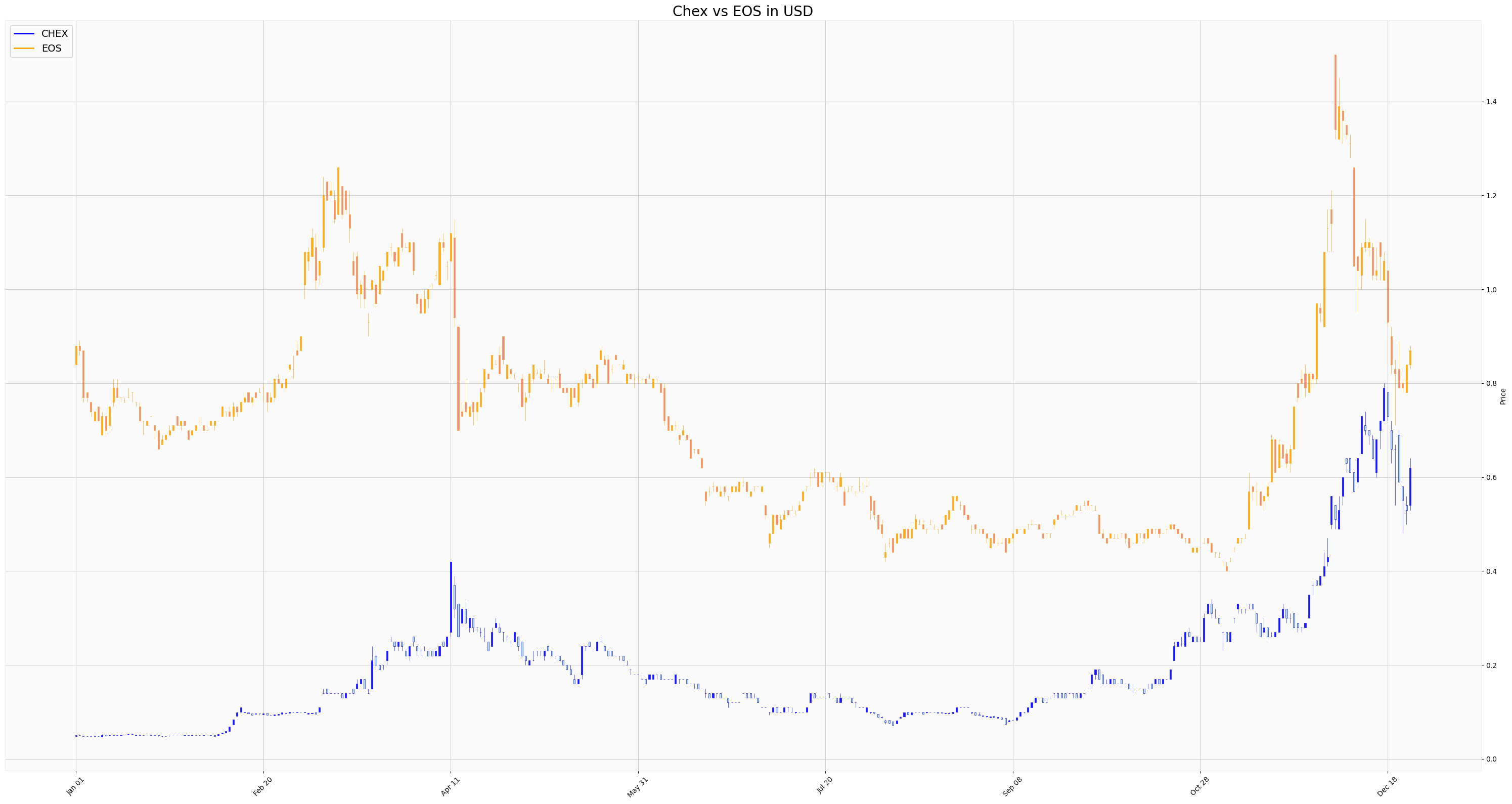
From there I calculated the price range being traded every day and plotted the result.
chex_df["Daily_Range"] = (chex_df["High"] - chex_df["Low"]).abs()
eos_df["Daily_Range"] = (eos_df["High"] - eos_df["Low"]).abs()

# Step 3: Merge data on Date for comparison
merged_ranges = pd.merge(chex_df[["Date", "Daily_Range"]], eos_df[["Date", "Daily_Range"]], on="Date", suffixes=("_Chex", "_EOS"))

# Step 4: Plot the daily range for both coins
plt.figure(figsize=(15, 8))
plt.plot(merged_ranges["Date"], merged_ranges["Daily_Range_Chex"], label="Chex Daily Range", color="blue", linewidth=2)
plt.plot(merged_ranges["Date"], merged_ranges["Daily_Range_EOS"], label="EOS Daily Range", color="orange", linewidth=2)
plt.title("Daily High-Low Range for Chex and EOS (Positive Values Only)", fontsize=16)
plt.xlabel("Date", fontsize=14)
plt.ylabel("Price Range", fontsize=14)
plt.xticks(fontsize=12)
plt.yticks(fontsize=12)
plt.legend(fontsize=12)
plt.grid(True, linestyle="--", alpha=0.6)
plt.tight_layout()
plt.show()
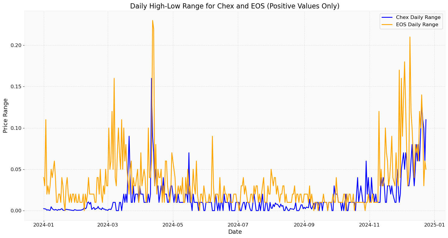
Next I plotted this daily range as a percentage of average price to get a better sense of the tokens' relative volatility.
chex_df["Daily_Average"] = (chex_df["High"] + chex_df["Low"]) / 2
chex_df["Range_Percentage"] = ((chex_df["High"] - chex_df["Low"]) / chex_df["Daily_Average"]) * 100

eos_df["Daily_Average"] = (eos_df["High"] + eos_df["Low"]) / 2
eos_df["Range_Percentage"] = ((eos_df["High"] - eos_df["Low"]) / eos_df["Daily_Average"]) * 100

# Step 3: Merge data on Date for comparison
merged_ranges = pd.merge(
    chex_df[["Date", "Range_Percentage"]],
    eos_df[["Date", "Range_Percentage"]],
    on="Date",
    suffixes=("_Chex", "_EOS")
)

# Step 4: Plot the range as a percentage of average price
plt.figure(figsize=(15, 8))
plt.plot(
    merged_ranges["Date"],
    merged_ranges["Range_Percentage_Chex"],
    label="Chex Range (%)",
    color="blue",
    linewidth=2
)
plt.plot(
    merged_ranges["Date"],
    merged_ranges["Range_Percentage_EOS"],
    label="EOS Range (%)",
    color="orange",
    linewidth=2
)
plt.title("Daily Range as Percentage of Average Price (Chex vs EOS)", fontsize=16)
plt.xlabel("Date", fontsize=14)
plt.ylabel("Range (%)", fontsize=14)
plt.xticks(fontsize=12)
plt.yticks(fontsize=12)
plt.legend(fontsize=12)
plt.grid(True, linestyle="--", alpha=0.6)
plt.tight_layout()
plt.show()
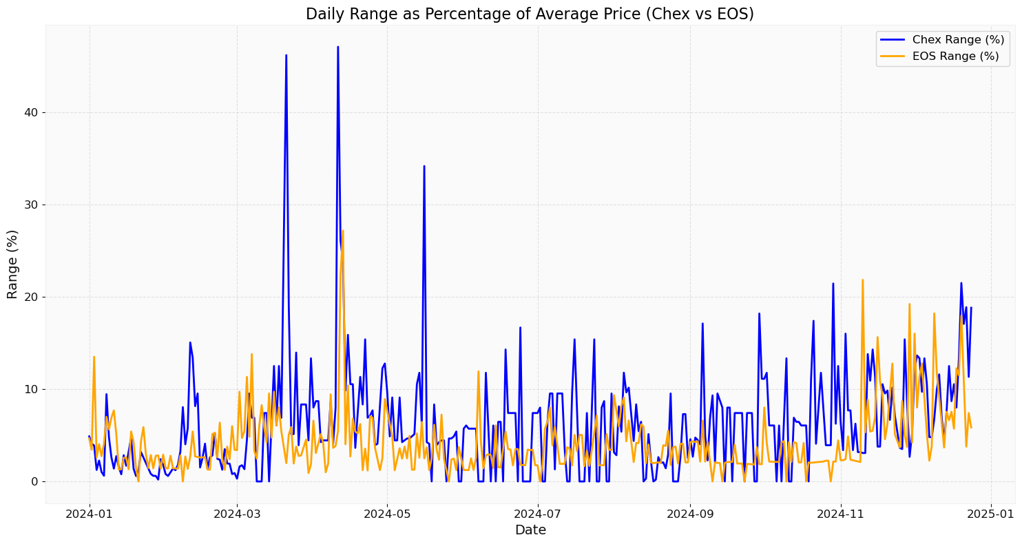
Probability
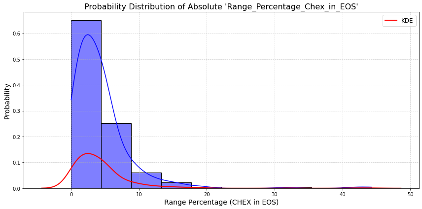
With the data firmly wrangled, I calculated the probabilities of volatility levels appearing. These results were very promising.
adj_df = adj_df.dropna(subset=["Range_Percentage_Chex_in_EOS"])

# Calculate absolute positive values for 'Range_Percentage_Chex_in_EOS'
adj_df["Range_Percentage_Chex_in_EOS"] = adj_df["Range_Percentage_Chex_in_EOS"].abs()

# Plot histogram with KDE overlay
plt.figure(figsize=(12, 6))
sns.histplot(
    adj_df["Range_Percentage_Chex_in_EOS"],
    bins=10,  # Number of bins
    kde=True,  # Add KDE
    stat="probability",  # Normalize to probabilities
    color="blue",  # Histogram color
)

# Add labels and title
plt.title("Probability Distribution of Absolute 'Range_Percentage_Chex_in_EOS'", fontsize=16)
plt.xlabel("Range Percentage (CHEX in EOS)", fontsize=14)
plt.ylabel("Probability", fontsize=14)
plt.grid(True, linestyle="--", alpha=0.6)

# Optional: Adjust KDE line appearance separately
sns.kdeplot(
    adj_df["Range_Percentage_Chex_in_EOS"],
    color="red",
    linewidth=2,
    label="KDE",
)

plt.legend(fontsize=12)
plt.tight_layout()
plt.show()
Simulation
With this info, I devised a trading strategy, then created a simulation with gpt's help to test this strategy. The underlying idea was that prices can't be predicted but volatility can, so an algo that anticipates big price swings could theoretically harvest more than an algo that just does simple market making or range trading. The initial algo I developed was a total failure.
After simulating the loss of my entire roll many times, I eventually just did a computationtionally intensive grid search of the entire parameter space to identify the right parameters for this algo on this pair. And suddenly, bam! A very promising algo emerged. Note that the sim begins with a bankroll of 1000 EOS.
# Initial setup
initial_eos = 1000
volatility_threshold_low =   # x% spread
volatility_threshold_high =   # x% spread
buy_spread =  # Adjusted buy spread
sell_spread =  # Adjusted sell spread
fee_rate = 0.01 # 1% trading fee
order_size_fraction =  # Use x% of available funds for each order

# Prepare historical data
data = food.copy()  # Use your DataFrame with necessary columns
data = data.sort_values("Date").reset_index(drop=True)

# Initialize variables for volatility strategy
eos_balance_volatility = initial_eos
chex_balance_volatility = 0
bankroll_volatility = []

# Initialize variables for buy-and-hold strategy
eos_balance_buyhold = initial_eos - 100  # Spend 100 EOS on CHEX
chex_balance_buyhold = 100 / data.loc[0, "Open_Chex_in_EOS"]  # Buy CHEX at day 1 open price
bankroll_buyhold = []

# Simulate trading
for i in range(1, len(data)):
    # Get previous day's close price
    prev_close = data.loc[i - 1, "Close_Chex_in_EOS"]

    # Determine spreads based on volatility
    spread = volatility_threshold_high / 100 if data.loc[i, "Range_Percentage_Chex_in_EOS"] >= 10 else volatility_threshold_low / 100

    # Calculate buy and sell prices with asymmetric spreads
    buy_price = prev_close * (1 - buy_spread)
    sell_price = prev_close * (1 + sell_spread)

    # Get today's open, high, low, close prices
    today_high = data.loc[i, "High_Chex_in_EOS"]
    today_low = data.loc[i, "Low_Chex_in_EOS"]
    today_close = data.loc[i, "Close_Chex_in_EOS"]

    # Adjust order size based on available funds
    eos_order_size = eos_balance_volatility * order_size_fraction
    chex_order_size = chex_balance_volatility * order_size_fraction

    # Execute trades
    # Sell CHEX if today's high >= sell_price
    if today_high >= sell_price and chex_balance_volatility > 0:
        sell_amount = chex_order_size
        eos_balance_volatility += sell_amount * sell_price * (1 - fee_rate)
        chex_balance_volatility -= sell_amount

    # Buy CHEX if today's low <= buy_price
    if today_low <= buy_price and eos_balance_volatility > 0:
        buy_amount = eos_order_size / buy_price
        eos_balance_volatility -= buy_amount * buy_price * (1 + fee_rate)
        chex_balance_volatility += buy_amount

    # Calculate total bankroll for volatility strategy
    total_bankroll_volatility = eos_balance_volatility + chex_balance_volatility * today_close
    bankroll_volatility.append(total_bankroll_volatility)

    # Buy-and-hold strategy
    total_bankroll_buyhold = eos_balance_buyhold + chex_balance_buyhold * today_close
    bankroll_buyhold.append(total_bankroll_buyhold)

# Final buy-and-hold adjustment
# Sell CHEX for EOS on the last day
eos_balance_buyhold += chex_balance_buyhold * data.loc[len(data) - 1, "Close_Chex_in_EOS"] * (1 - fee_rate)
chex_balance_buyhold = 0
final_bankroll_buyhold = eos_balance_buyhold

# Plot results
plt.figure(figsize=(14, 7))
plt.plot(data["Date"][1:], bankroll_volatility, label="Volatility Strategy", color="blue", linewidth=2)
plt.plot(data["Date"][1:], bankroll_buyhold, label="Buy and Hold", color="orange", linewidth=2)
plt.title("Trading Strategy Simulation: Volatility vs Buy-and-Hold", fontsize=16)
plt.xlabel("Date", fontsize=14)
plt.ylabel("Total Holdings (EOS Equivalent)", fontsize=14)
plt.grid(True, linestyle="--", alpha=0.6)
plt.legend(fontsize=12)
plt.tight_layout()
plt.show()

# Print final bankrolls
print(f"Final Volatility Strategy Bankroll: {bankroll_volatility[-1]:.2f} EOS")
print(f"Final Buy-and-Hold Strategy Bankroll: {final_bankroll_buyhold:.2f} EOS")
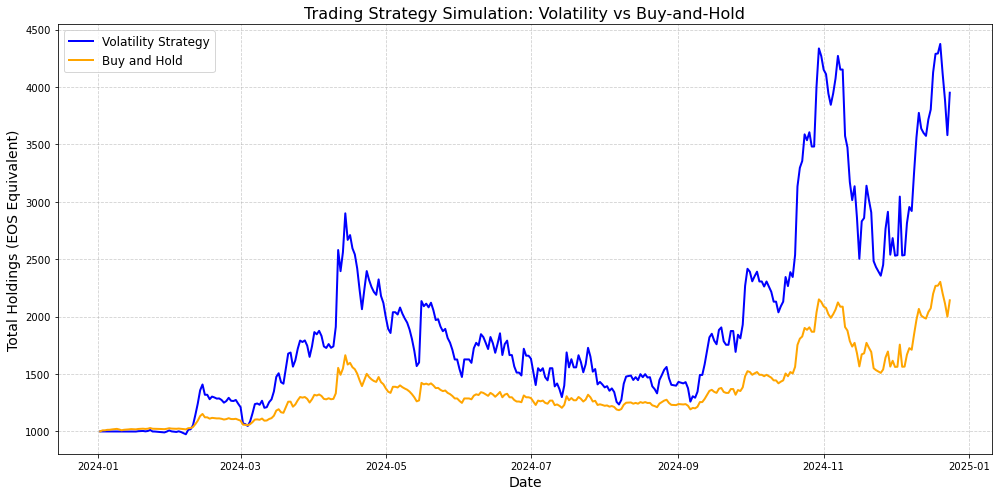
Final Volatility Strategy Bankroll: 3949.95 EOS
Final Buy-and-Hold Strategy Bankroll: 2129.53 EOS
Next Steps
My next steps include waiting for Newdex to provide me with an api key, generalizing my method into a scale-free approach to automated trading on any high-volatility pair, and manually trading using this strategy to see how it performs in the unpredictable real world. If you're making trading bots and you want to compare notes, hit me up.
Read Free Mind Gazette on Substack
Read my novels:
- Small Gods of Time Travel is available as a web book on IPFS and as a 41 piece Tezos NFT collection on Objkt.
- The Paradise Anomaly is available in print via Blurb and for Kindle on Amazon.
- Psychic Avalanche is available in print via Blurb and for Kindle on Amazon.
- One Man Embassy is available in print via Blurb and for Kindle on Amazon.
- Flying Saucer Shenanigans is available in print via Blurb and for Kindle on Amazon.
- Rainbow Lullaby is available in print via Blurb and for Kindle on Amazon.
- The Ostermann Method is available in print via Blurb and for Kindle on Amazon.
- Blue Dragon Mississippi is available in print via Blurb and for Kindle on Amazon.
See my NFTs:
- Small Gods of Time Travel is a 41 piece Tezos NFT collection on Objkt that goes with my book by the same name.
- History and the Machine is a 20 piece Tezos NFT collection on Objkt based on my series of oil paintings of interesting people from history.
- Artifacts of Mind Control is a 15 piece Tezos NFT collection on Objkt based on declassified CIA documents from the MKULTRA program.