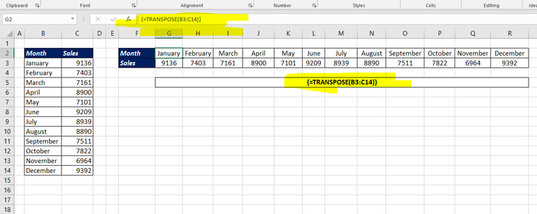
If your data is supposed to change you should go for an Array formula using TRANSPOSE function. The array formula for the example shown in the screenshot is
{=TRANSPOSE(B3:C14)}
Now about how to enter this formula.
Select the cells from G2 to R3, Type in the formula =TRANSPOSE(B3:C14) and press CTRL, SHIFT and ENTER keys together. A pair of braces will be added to your formula and the data present in the cells from B3 to C14 will be transposed into the selected cells.
One more example for your understanding
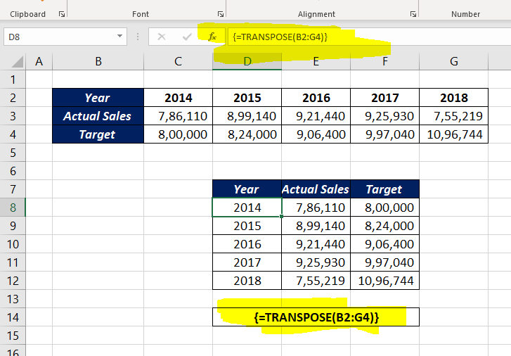
To transpose the data present in the cells B2 to G4 into the cells D7 to F12,
Select the cells from D7 to F12, Type in the formula =TRANSPOSE(B2:G4) and press CTRL, SHIFT and ENTER keys together.


did you know in Excel 365 you don't need to press CTRL, SHIFT and ENTER? Excel sees everything as arrays in Excel 365