The ability to customize the Excel ribbon is a great way to enhance your workflow, improve on your productivity or simply to give the platform a unique feel to it. In the following article we will uncover three topics:

Ways to hide and unhide the ribbon menu
How to customize your ribbon
Resetting all customization to default

Basic overview

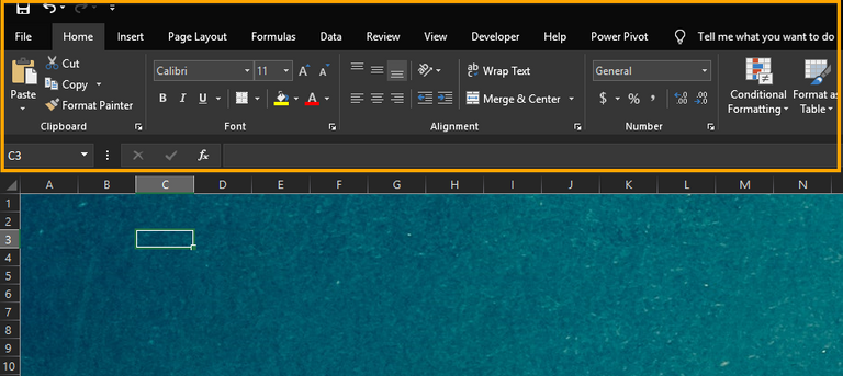
The Excel ribbon is a batch of icons above the Excel worksheet UI. It's a complex toolbar, which purpose is to replace the menu toolbar and be able to reach the functions much quicker.

Above the ribbon are the Excel tabs (Home, Insert, etc.). Clicking a tab initiates the Excel ribbon category which contains collections of icons for different purposes.

Home tab is set as a default when Excel opens, it contains common grouped commands, like Fonts, Clipboard, etc.

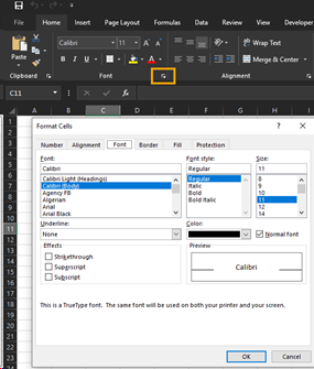
Each group command has a button in the lower-right corner that opens a dialog box containing further options related to that group. For example, the dialog box button on the Font group opens the Font Settings dialog box.

Ways to hide and unhide the Excel ribbon

You can hide (collapse) and show the Excel ribbon in order to increase the available space for your worksheet. This is particularly helpful when you work on a laptop with a smaller screen.

Hide the Excel Ribbon

There are three main ways to collapse the Excel ribbon.

The first option is to click the up arrow button in the lower-right corner of the ribbon

The second option to collapse it is using the shortcut key Ctrl+F1
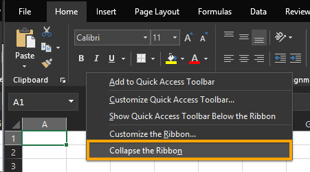
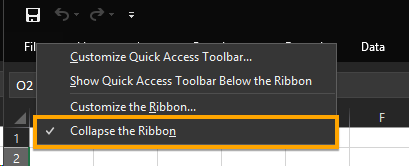
The third option is to is to right-click on the ribbon and choose to Collapse the Ribbon.

Automatically Hide the Excel Ribbon

You have the ability to automatically hide the entire ribbon, including the tabs to maximize the available workspace.

To automatically hide the ribbon and the tabs, you will find the Ribbon Display Options button in the upper-right corner of the Excel window where you can select Auto-hide Ribbon option from the dropdown menu

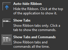
To keep the tabs options but hide the ribbon, choose the Show Tabs option from the dropdown menu
To permanently show the tabs and the ribbon again, select Show Tabs and Commands* option.
To temporarily show the tabs and the ribbon again, hover your mouse over the top of the Excel window until you see the highlighted bar and click on the bar. (The ribbon will automatically hide again as soon as you choose a command)

Show the Excel Ribbon

In order to temporarily show the ribbon again, click one of the Excel tabs and the ribbon will appear until you pick a function from the tab.

If you want to permanently show the ribbon again, you can do it one of the following ways:

double-click an Excel tab bar with your mouse cursor
use the keyboard shortcut key Ctrl + F1
right-click on the tab bar and select Collapse the Ribbon

Customize the Excel Ribbon

Recent Excel versions have the ability to customize the ribbon to your personal needs, we will look into how to:

Add a new Group to the Ribbon
Add a Command to a New Group
Create your own Custom Tab
Rearrange Tabs, Groups, and Commands
Hide tabs on Excel Ribbon
Rename the items on the Ribbon
Use only Icons on the Ribbon

Keep in mind that you can’t change or delete default Excel commands, icons or names, or changing the order of the default commands.

To customize the ribbon, right-click on the ribbon and select Customize the Ribbon. You can also go to File > Options > Customize Ribbon or right click on the ribbon and choose to Customize Ribbon.

Add a new Group to the Ribbon

Every command located in the ribbon has to be classified in groups. If you want to add a command to an existing tab, you have to create a new group or add to an existing customized group which I'll show you how to do.

There may be some commands hidden away which you would prefer to be available on the ribbon:

Go to the Excel dialog box > Customize the Ribbon screen and choose the Commands Not in the Ribbon from the Choose commands dropdown list on the left.
Select Main Tabs from the Customize Ribbon dropdown list on the right.

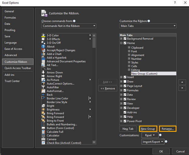
Excel won't let you add commands to existing groups on the Main Tabs. For that, you will need to create a new group. In this example we want to add the new command to the Home tab, therefore, we select the Home tab in the list on the right and then click New Group from the list.

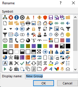
-You can Rename your new group and give it a symbol by right-clicking on it and choosing Rename, or selecting the group and choose Rename from the dialog box

Add a Command to a New Group

Once you created a new group, you can add commands to it.

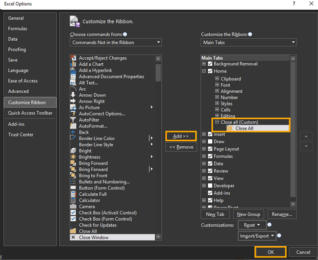
Choose the group from the right side of the dialog box and select the commands you want to add into the group from the left side of the dialog box. Click Add.

Create your own Custom Tab

You learned how to add groups and commands to the existing tabs, now you can learn how to create your own custom tabs.
For example, I use this when I need my most used macros to be easily accessible.

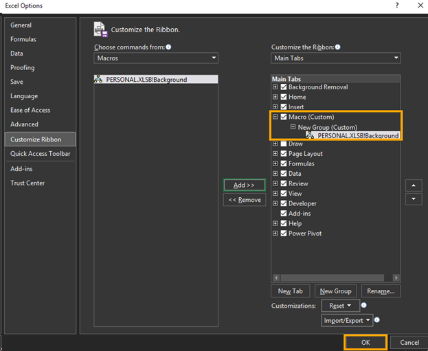
Go to the Excel dialog box > Customize the Ribbon screen and choose Macros from the Choose commands dropdown list on the left of the window.
Select Main Tabs from the Customize Ribbon dropdown list on the right
Choose Newly created Tab
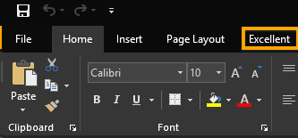
Highlight your new tab and click Rename. I renamed mine to Macro.
Add your macros from the left side (If you want know how to create a quick macro, check out this article

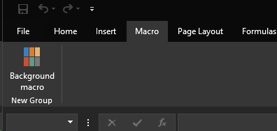
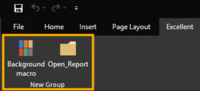
Press OK to return to the spreadsheet where you can see the Macro custom tab and the macro shortcut in it.

Rearrange Tabs, Groups, and Commands

If you want to move tabs, groups, or commands, go to Excel Options dialog box and select Customize the Ribbon screen.

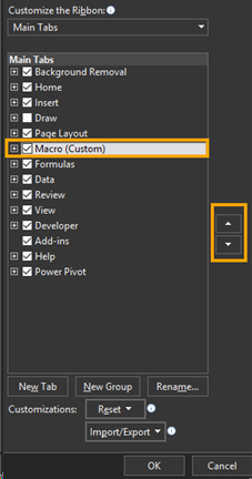
On the right of the screen, select the tab, group, or command which you want to move and then click the up or down arrow to the right of the list to move it each way.
Tabs on top of the list are displayed on the far left side of the Excel ribbon, while the tabs at the bottom on the far right.

Hide tabs on Excel Ribbon

You have the option to hide tabs which you don't use and make the Excel workspace customized to your needs.

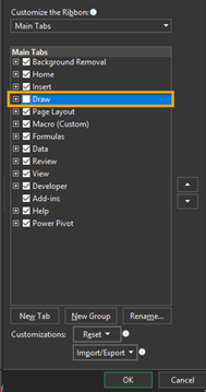
Go to Customize the Ribbon and on the right side of the window, uncheck the boxes for tabs you want to hide. Then, click OK.

Rename the items on the Ribbon

You can rename your custom tabs and groups you made, but keep in mind that you can’t rename default commands on the ribbon.

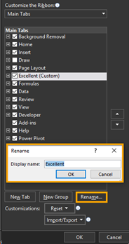
Go to Customize the Ribbon and on the right side of the window, select the group you want to rename. Click Rename button below the list. On the Rename dialog box, enter the name you want and click OK.

Use only Icons on the Ribbon

There are situations when the use of icons only ribbon makes sense. For example, if you use a laptop with a small screen, you can save some space by removing the text from custom groups and commands with certain limitations:

You can’t remove the text from built-in commands on the main tabs.
You must remove the text from all the icons in a custom group, not just one of them.

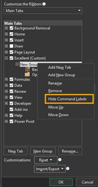
Go to Customize the Ribbon and on the right side of the window, right click on the excel group you want to change and select Hide Command Labels.

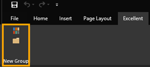
The commands in your custom group will display without text now.

Resetting Customizations in Excel

In case you made a lot of customizations to the Excel ribbon, and you want to reverse back to the default order,

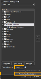
Go to Customize the Ribbon window and on the right side, click the Reset button and select Reset all customization. (This option also resets the quick action toolbar to its default settings). Click Yes to confirm.

How to customize your Excel Ribon and increase your productivity