So, in my first post about CAs I discussed setting up an elementary CA - a simple 1-dimensional row of "cells". In this post I want to follow up with a discussion of what it takes to set up a more common 2-D CA, specifically the most famous one of them all - Conway's Game of Life CA.
Once we are done, you will be able to run a simulation shown in this video or the preview below .
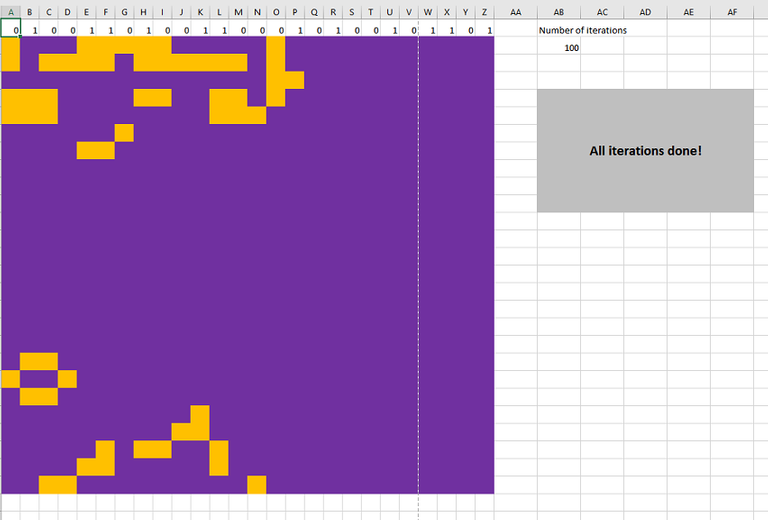
(preview from the video)
If that looks like fun, let's delve into the implementation.
By way of a reminder, the defining feature of the elementary CA was its 1-dimensional nature - it was just a single row of cells. However, what we ended up with while simulating traffic flow using Rule 184 was a grid of cells. How did that happen? Well, we simply added a time dimension - so you could see how that first top row of cells was changing as Rule 184 was successively applied to the preceding row. This worked well for us in simulating a time series of the flow of traffic. However, when we start out with a 2-D CA, this trick no longer works. We have to actually keep a separate copy of the entire 2-D grid so we can apply the rules "in parallel" - at least logically. Once the rules are all applied a completely new 2-D grid of CA cells replaces the old one. That's how higher-dimensional CAs work.
So, let's see how we can do this in Excel.
Fire up a new Excel workbook and set up the first row of A to Z cells as follows:
A1 - type in "=randbetween(0,1)". Drag lower left hand corner cross hairs of A1 across to Z1
Like before we are going to use this first top row to "seed" the initial configuration of the CA. Unlike the elementary CA where we seeded just the initial top row (that was the entire CA), in this case we will copy a random configuration down however many rows our CA is meant to have. In this particular case let us do a 26x26 square (columns A-Z across, and rows 2-27 down).
Select cell A5 and drag down the selection to AF11. Click on "Merge and Center". Set the vertical and horizontal alignment to "center", set the fill color to light gray, and make the font bold, Calibri, size 16.
This will be our custom status tableau.
Click on View tab and on the "Macros" submenu.
Type in "SetupData" in the prompt window. This should enable the "Create" button, which you can now click on.
This will open up the VBA Editor and setup the sub[routine] SetupData().
Paste the code below between the beginning and ending of the subroutine, so that the whole thing looks like this.
Sub SetupData()

SetEnv
Range("AB5").Value = "Initializing..."
Range("A2:Z42").Select
Selection.ClearContents
For x = 1 To 26
Range("AB5").Value = "Initializing row " + Str(x)

Calculate
Range("A1:Z1").Select
Selection.Copy
Range("A1").Select

Cells.Find(What:="", After:=ActiveCell, LookIn:=xlFormulas, LookAt:= _
    xlWhole, SearchOrder:=xlByColumns, SearchDirection:=xlNext, MatchCase:= _
    False, SearchFormat:=False).Activate

Selection.PasteSpecial Paste:=xlPasteValues, Operation:=xlNone, SkipBlanks _
    :=False, Transpose:=False

DoEvents
Next x
ResetEnv
Range("AB5").Value = "Initialization Complete!"


End Sub
Place your mouse cursor after the "End Sub" and press Enter a few times. Then copy and paste the following code. (You might have noticed that these two subroutines get called at the beginning and the end of the SetupData subroutine - they are used to speed up the execution by disabling some features of Excel and then re-enabling them again).
Sub SetEnv()


Application.Calculation = xlCalculationManual
' Application.ScreenUpdating = False
Application.DisplayStatusBar = False
Application.EnableEvents = False
ActiveSheet.DisplayPageBreaks = False

End Sub

Sub ResetEnv()

Application.Calculation = xlCalculationAutomatic
Application.ScreenUpdating = True
Application.DisplayStatusBar = True
Application.EnableEvents = True
ActiveSheet.DisplayPageBreaks = True

End Sub
Click on the "Save" button and close the VBA window. Click on "View Macros" again. You should see 3 macros now in the dialogue box - "SetupData", "SetEnv" and "ResetEnv". Select "SetupData" and click on "Options". Let's give it a shortcut - CTRL+g. Close the dialogue box.
To test if everything is working simply press CTRL+g. You should be seeing a bunch of 0's and 1's being added sequentially down through row 27.
In order to make this look a bit more compelling let's add some formatting.
Select the range A2:Z27. While on the Home tab, click on "Conditional formatting". We will add 2 new rules. The first rule will be using icon sets and it should look like the pic.1 below:
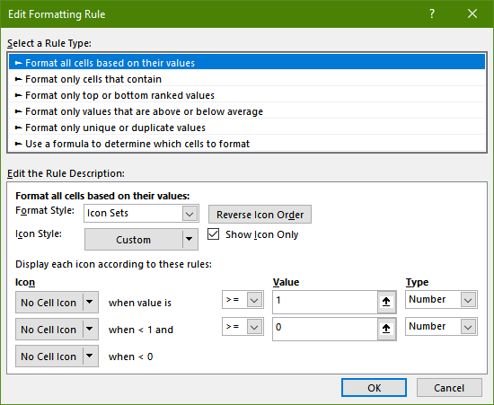
Pic.1
This will hide the actual 0s and 1s in the cells.
Click "OK and add the following rule (pic.2):
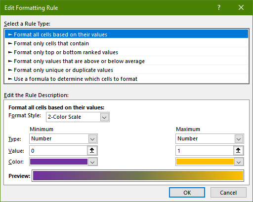
Pic.2
Click "OK" and then "OK" again to save the new formatting rules.
Now select the columns A-Z, right-click and select "Column width". Set that to 3.25. Select row headers 2-27, right click and choose "Row height". Set that to 20.
After these changes your screen should resemble the following screenshot (pic.3):
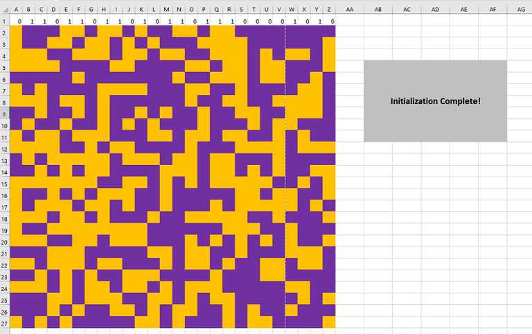
Pic.3
Now for the final pièce de résistance - the actual code for the CA.
On the View tab, click on "Macros" and then on "View Macros" button. Type in "Game_of_Life" and click on "Create". Paste the code below so that you have a sub[routine] that looks like this:
Sub Game_of_Life()
'
'
' Keyboard Shortcut: Ctrl+l
'
Dim CellData As Variant
Dim rowOffset As Integer
Dim colOffset As Integer
Dim rangeWidth As Integer
Dim rangeHeight As Integer

Dim leftCell As Integer
Dim rightCell As Integer
Dim selfCell As Integer

Dim upperLeftCell As Integer
Dim lowerLeftCell As Integer
Dim upperRightCell As Integer

Dim lowerRightCell As Integer
Dim upperSelfCell As Integer
Dim lowerSelfCell As Integer

Dim left_coord As Integer
Dim right_coord As Integer
Dim top_coord As Integer
Dim bottom_coord As Integer
Dim sumNeighbors As Integer

Dim iterations As Integer

iterations = Range("AB2").Value2

rowOffset = 2
colOffset = 1
rangeWidth = 26
rangeHeight = 26

SetEnv

For Z = 1 To iterations

    Range(Cells(rowOffset, colOffset), Cells(rowOffset + rangeHeight - 1, colOffset + rangeWidth - 1)).Select

    CellData = Selection.Value2

    Range("A1").Select

    Range("AB5").Value = "Game of Life: Iteration # " + Str(Z)

    For x = 1 To rangeHeight

        For y = 1 To rangeWidth

            selfCell = CellData(x, y)

            'defaults
            left_coord = y - 1
            right_coord = y + 1
            top_coord = x - 1
            bottom_coord = x + 1

            ' corner case - literally, in the left corner
            If y = 1 Then
                left_coord = rangeWidth
            End If

            ' corner case - literally, in the right corner
            If y = rangeWidth Then
                right_coord = 1
            End If

            ' corner case - top row
            If x = 1 Then
                top_coord = rangeHeight
            End If

            ' corner case - bottom row
            If x = rangeHeight Then
                bottom_coord = 1
            End If

            leftCell = CellData(x, left_coord)
            rightCell = CellData(x, right_coord)

            upperLeftCell = CellData(top_coord, left_coord)
            lowerLeftCell = CellData(bottom_coord, left_coord)

            upperRightCell = CellData(top_coord, right_coord)
            lowerRightCell = CellData(bottom_coord, right_coord)

            upperSelfCell = CellData(top_coord, y)
            lowerSelfCell = CellData(bottom_coord, y)

            sumNeighbors = leftCell + rightCell + upperLeftCell + lowerLeftCell + upperRightCell + lowerRightCell + upperSelfCell + lowerSelfCell

            ' rule Game of Life
            If (selfCell = 0 And sumNeighbors < 3) Or (selfCell = 1 And sumNeighbors > 3) Or (selfCell = 1 And sumNeighbors < 2) Then
                ActiveSheet.Cells(x + rowOffset - 1, y + colOffset - 1).Value = 0
            ElseIf (selfCell = 0 And sumNeighbors = 3) Or (selfCell = 1 And sumNeighbors = 3) Or (selfCell = 1 And sumNeighbors = 2) Then
                ActiveSheet.Cells(x + rowOffset - 1, y + colOffset - 1).Value = 1
            Else
                ActiveSheet.Cells(x + rowOffset - 1, y + colOffset - 1).Value = 0
            End If

        Next y

        DoEvents

    Next x

Next Z

ResetEnv

Range("AB5").Value = "All iterations done!"

End Sub
Save the subroutine and close the VBA window. Now click on "Macros" again, select "Game_of_Life" and click on "Options". Let's give it a shortcut CTRL+L. Close the dialogue box.
In cell AB1 type in "Number of iterations". In cell AB2 type in "100" - our initial # of iterations to run.
OK, are you ready for the big moment???
Hit CTRL+L.
You should be seeing something similar to what was recorded in the video at the beginning of the post or on pic.4 below.

Pic.4