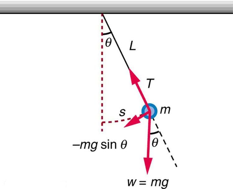
Here is a free-body diagram of a simple pendulum from which physics, engineers and mathematicians can formulate its equation of motion.
 Image Source
Solving the equation of motion, the period of oscillation a simple pendulum is usually given by...

More precisely, the expression should be...

However, mathematicians throughout history (who are notorious for always looking for shortcuts) have noted that...

...for small angles of θ. And thus, the θ and the sinθ terms in the above equation can cancel themselves out.
The author of Physics: Calculus 2nd Edition Eugene Hecht states in his book:
"for small angles, the value of θ in radians is very nearly the value of sinθ; they differ by less than 2% out to about 20°
In this tutorial, let's verify by linear approximation that...

...near x = 0. Let's also find out how what values of x where sinx and x differ by less than 2%.
So, for...

Its derivative is...

And evaluating these at x = 0, we have...


And putting these into the tangent line formula yields...

Thus our linear approximation for sinx is L(x) = x. Therefore, we have shown that when x is near 0...

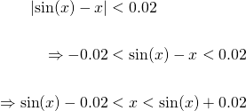
Good. We've got the answer to the first part of our question. Now to answer the second part, we need the difference between x and sinx to be less than 0.02. Thus...

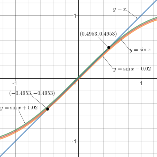
Now, if we investigate this graphically...

Created with: www.desmos.com/calculator
Note that the blue line is y = x, the red curve is y = sinx, the green curve is y = sinx + 0.02 and the orange curve is y = sinx - 0.02.
As we can see, y = x is indeed a good approximation of y = sinx near x = 0. The blue line intersects the green and orange curves at x = -0.495 and x = 0.495 radians respectively.
We can conclude that...

...for x to be within 2% of sinx, which means we can swing the pendulum quite far and conveniently use x in the place of sinx. I'll show why this is significant in a future post.
Here's a list of posts created so far on the subject of Linear Approximations and Differentials:
- Linear Approximations Part 1 - Interpolating between Empirical Data
- Linear Approximations Part 2 - Estimating values of f(x) = √(x+2) near x = 2
- Linear Approximations Part 3 - why sin(x) ≅ x near 0
Please give me an Upvote and Resteem if you have found this tutorial helpful.
Please ask me a maths question by commenting below and I will try to help you in future videos.
I would really appreciate any small donation which will help me to help more math students of the world.
Tip me some DogeCoin: A4f3URZSWDoJCkWhVttbR3RjGHRSuLpaP3
Tip me at PayPal: https://paypal.me/MasterWu
A nice treatment of limits like sin(x), x-> 0 can be found here:
https://ocw.mit.edu/courses/mathematics/18-01-single-variable-calculus-fall-2006/video-lectures/lecture-3-derivatives/
In particular, he illustrates sin(x) vs. the chord for small angles, which makes it obvious geometrically that the limit is the angle for small angles (since the circular arc and chord end up approaching each other).
Thanks for your comment @peeterjoot. I will discuss the sin(x) vs. the chord problem in a future post. Thanks again for reminding me.
Thank you @steemiteducation!
@originalworks
To call @OriginalWorks, simply reply to any post with @originalworks or !originalworks in your message!